The design of a wind farm encompasses many complex steps, from the selection of the most adequate turbine model to their optimum location in the available land and, moreover, the prediction of its future production: farms are usually designed for a lifespan of 20-25 years. In some cases, and considering the limitations imposed by regulation, terrain characteristics or any other financial or physical constraint, the optimum size of the wind farm is also a subject of study. The difficulty of the design work comes from the fact that we only have a limited set of data to accomplish this goal, and the most reliable dataset, the one recorded onsite, is limited to a few year’s period and a few spots around the site. So, how can analysts estimate the adequate size of the wind farm and where to locate the turbines to optimise production? 

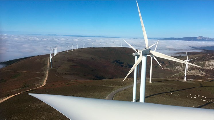
For all of these questions, CFD models applied to resolve the dynamics of the atmospheric boundary layer are of a crucial relevance. When the project design begins, wind analysts have wind observations recorded at some specific locations in the wide area previously selected for a future plant. As a rule of thumb, precision in the prediction of the farm energy production will increase with the number of wind measurement instrumentation available. However, their number rarely ever equals the number of potential turbines to be installed, and therefore, an accurate wind model providing estimates is needed to extrapolate from this limited dataset. If terrain characteristics are simple (flat terrain and absence of big obstacles like woods), simple approximations can be used, but when things get complicated, like in steep terrain with woods or locations with complex atmospheric-surface interactions, CFD models are mandatory (see an example of a complex wind farm in Fig. 1). Their capacity to resolve these features makes of them a key tool to be used in these cases.

Within ENERXICO, our intention is to include characteristics of the wind flow that belongs to scales well above the size of a wind farm into the CFD simulations. This approach will increase the accuracy of simulations, since local flow is usually influenced by the dynamics of mesoscale and synoptic scales, although this information is not realistically included in CFD models. The mesoscale dynamics are resolved by means of the model WRF (Weather Research and Forecasting), that uses as input the information contained in global models (e.g. ERA5). Global models resolve the large scale dynamics over coarser grids (around 30 km), that are downscaled to a few kilometers with the help of WRF (typically 3 to 1 km). Therefore, by using WRF and coupling it to a CFD model we try to effectively make use of the information in the cascade from large scale dynamics to local microscale characteristics of the wind flow over the wind farm.

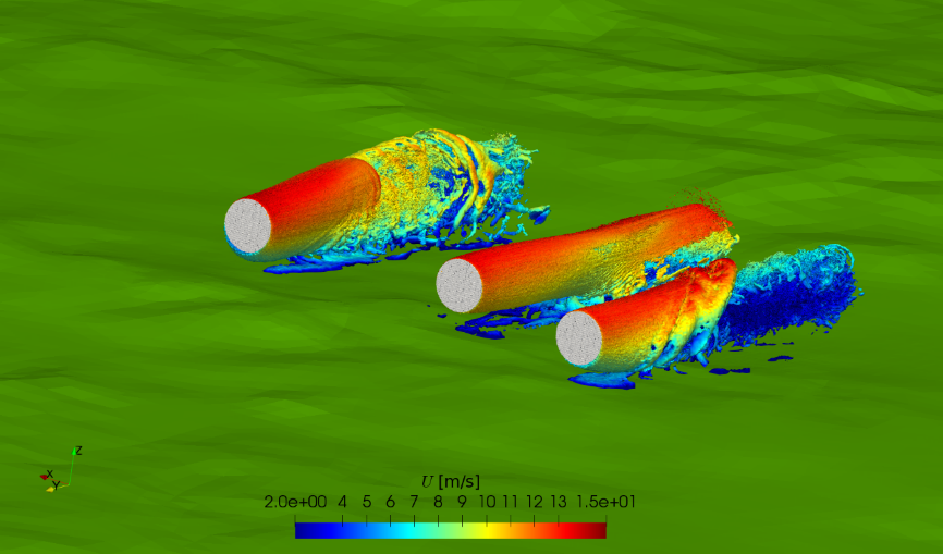
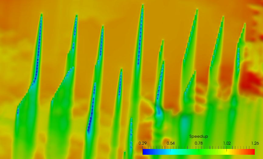
It is crucial to this project to bear in mind the increase of computational resources needed to successfully use these cutting-edge methodologies. Typically, a CFD like the one that runs at BSC (Barcelona Supercomputing Center) for wind farm design (CFD Alya, a RANS model, see Figure 2 for an example) can resolve the flow over a standard farm in around 100.000 CPU hours. Using a dynamical coupling technique to link both models (WRF for the mesoscale and CFD Alya for the micro), can multiply the computational cost by 150, which means that we would need to use the whole capacity of a supercomputing like Marenostrum 4 at BSC to have results in a reasonable amount of time (4 days of computation time!). If we decided to use an even more complex microscale model such LES, the cost would be increased by 1000 (see figure 3 for an example of LES output). That gives nearly one month of computational time using the complete capacity of Marenostrum 4. If the figures displayed by a single case are already remarkable, just of think of how many potential wind farms a company like Iberdrola can analyse a year, meaning how many times a wind flow model could be used: around 50 cases. That places the scope of the project within the boundaries of exascale, since we need to dramatically increase the computation speed to make this approach something affordable for industrial applications.

The use of such a complex wind flow model would represent an outstanding breakthrough, but we are aware that it won’t be ready for industrial deployment in the short run, particularly because of the expensive computational cost, as explained beforehand. To avoid this limitation, we also pretend to develop methods that limit the amount of resources needed, keeping the core concept of the coupling. Particularly, we try to extract those key features of mesoscale dynamics that are worth used as inputs to the microscale model, restricting the coupled runs to a smaller sample of events that represent the local characteristics of wind flow. As part of a benchmark exercise to compare different approaches to wind flow modelling, we also intend to run CFD models with and without coupling, and also use commercial suits to compare results in terms of precision and costs, so we can fully understand the improvement in the use of such approximations, providing a snapshot on the cost of models and their associated precision gains in some actual wind farms.